728x90
반응형
사전 훈련된 네트워크(pretrained network)
- 일반적으로 대규모 이미지 분류 문제를 위해 대량의 데이터셋에서 미리 훈련되어 저장된 네트워크
VGG16
- 캐런 시몬연(Karen Simonyan)과 앤드류 지서먼(Andrew Zisserman)이 2014년에 개발한 VGG16 구조
- VGG16은 간단하고 ImageNet 데이터셋에 널리 사용되는 컨브넷 구조
- 최고 성능은 아니고 최근의 다른 모델보다는 무겁다.
- 케라스 패키지로 포함
- kears.applications 모듈에서 임포트 가능
- kears.applications에서 사용 가능한 이미지 분류 모델
- Xception
- Inception V3
- ResNet50
- VGG16
- VGG19
- MobileNet
사전 훈련된 네트워크 사용하는 두 가지 방법
- 특성 추출(feature extraction)
- 미세 조정(fine tuning)
특성 추출
- 사전에 학습된 네트워크의 표현을 사용해 새로운 샘플에서 흥미로운 특성을 뽑아내는 것
VGG16 모델
# VGG 합성곱 기반 층 만들기

from tensorflow.keras.applications import VGG16

conv_base = VGG16(weights='imagenet',
                 include_top=False,
                 input_shape=(150,150,3))
- VGG16 3개의 매개변수
- weight는 모델을 초기화할 가중치 체크포인트(checkpoint)를 지정한다.
- include_top은 네트워크의 최상위 완전 연결 분류기를 포함할지 안 할지 지정한다.
- input_shape은 네트워크에 주입할 이미지 텐서의 크기다. - 이 매개변수는 선택 사항
conv_base.summary()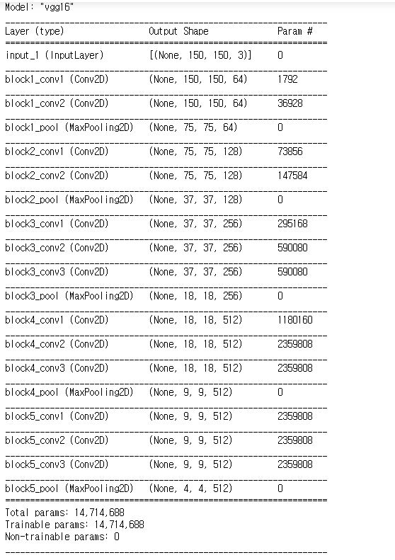
데이터 증식 사용하지 않는 빠른 특성 추출
# 사전 훈련된 합성곱 기반 층을 사용한 특성 추출

import os
import numpy as np
from tensorflow.keras.preprocessing.image import ImageDataGenerator

base_dir = './datasets/cats_and_dogs_small'
train_dir = os.path.join(base_dir, 'train')
validation_dir = os.path.join(base_dir, 'validation')
test_dir = os.path.join(base_dir, 'test')

datagen = ImageDataGenerator(rescale=1/255.0)
batch_size = 20

def extract_features(directory, sample_count):
    features = np.zeros(shape=(sample_count, 4, 4, 512))
    labels = np.zeros(shape=(sample_count))
    generator = datagen.flow_from_directory(
        directory,
        target_size=(150,150),
        batch_size = batch_size,
        class_mode='binary'
    )
    i = 0
    for inputs_batch, labels_batch in generator:
        features_batch = conv_base.predict(inputs_batch)
        features[i * batch_size : (i+1) * batch_size] = features_batch
        labels[i * batch_size : (i + 1) * batch_size] = labels_batch
        i+=1
        if i * batch_size >= sample_count :
            break
    return features, labels

train_features, train_labels = extract_features(train_dir, 2000)
validation_features, validation_labels = extract_features(validation_dir, 1000)
test_features, test_test_labels = extract_features(test_dir, 1000)


train_features = np.reshape(train_features, (2000, 4*4*512))
validation_features = np.reshape(validation_features, (1000, 4 * 4* 512))
test_features = np.reshape(test_features, (1000, 4*4*512))
완전 연결 분류기 정의 및 훈련
# 완전 연결 분류기 정의 및 훈련
from tensorflow.keras import models, layers, optimizers

model = model.Sequential()
model.add(layers.Dense(256, activation='relu',
                      input_dim = 4*4*512))
model.add(layers.Dropout(0.5))
model.add(layers.Dense(1, activation='sigmoid'))

model.compile(optimizer = optimizers.RMSprop(lr=2e-5),
            loss = 'binary_crossentropy',
             metrics = ['acc'])

log = model.fit(train_features, train_labels,
               epochs = 30,
               batch_size = 20,
               validation_data = (validation_features, validation_labels))
결과 그래프
# 결과 그래프 그리기

import matplotlib.pypolt as plt

acc = log.history['acc']
val_acc = log.history['val_acc']
loss = log.history['loss']
val_loss = log.history['val_loss']

epochs = range(1, len(acc) + 1)

plt.plot(epochs, acc, 'bo', label='Training acc')
plt.plot(epochs, val_acc, 'b', label='Validation acc')
plt.title('Training and Validation accuracy')
plt.legend()

plt.figure()

plt.plot(epochs, loss, 'bo', label = 'Training loss')
plt.plot(epochs, val_loss, 'b', label = 'Validation loss')
plt.title('Training loss and Validation loss')
plt.legend()

plt.show()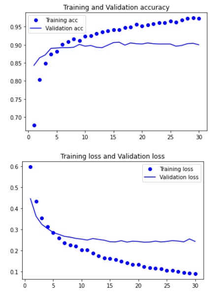
- 점점 과대적합되고 있다는 것을 보여준다.
데이터 증식을 사용한 특성 추출
- conv_base 모델을 확장하고 입력 데이터를 사용해 엔드-투-엔드로 실행
합성곱 기반 층 위에 완전 연결 분류기 추가
# 합성곱 기반 층 위에 완전 연결 분류기 추가

from tensorflow.keras import models, layers

model = models.Sequential()
model.add(conv_base)
model.add(layers.Flatten())
model.add(layers.Dense(256, activation='relu'))
model.add(layers.Dense(1, activation='sigmoid'))

model.summary()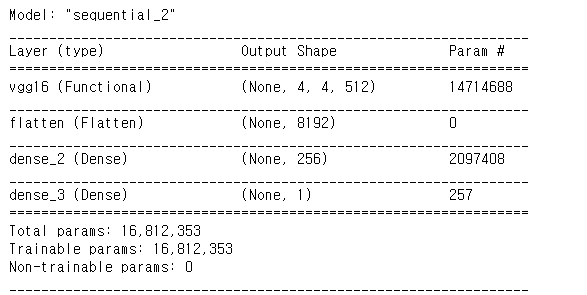
# trainable 속성을 False로 설정해 네트워크 동결

print('conv_base 동결 전 훈련 가중치 수 : ', len(model.trainable_weights))
conv_base.trainable= False
print('conv_base 동결 후 훈련 가중치 수 : ', len(model.trainable_weights))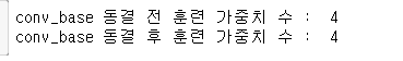
from tensorflow.keras.preprocessing.image import ImageDataGenerator

train_datagen = ImageDataGenerator(
      rescale=1./255,
      rotation_range=20,
      width_shift_range=0.1,
      height_shift_range=0.1,
      shear_range=0.1,
      zoom_range=0.1,
      horizontal_flip=True,
      fill_mode='nearest')

# 검증 데이터는 증식되어서는 안 됩니다!
test_datagen = ImageDataGenerator(rescale=1./255)

train_generator = train_datagen.flow_from_directory(
        # 타깃 디렉터리
        train_dir,
        # 모든 이미지의 크기를 150 × 150로 변경합니다
        target_size=(150, 150),
        batch_size=20,
        # binary_crossentropy 손실을 사용하므로 이진 레이블이 필요합니다
        class_mode='binary')

validation_generator = test_datagen.flow_from_directory(
        validation_dir,
        target_size=(150, 150),
        batch_size=20,
        class_mode='binary')

model.compile(loss='binary_crossentropy',
              optimizer=optimizers.RMSprop(lr=2e-5),
              metrics=['acc'])

history = model.fit_generator(
      train_generator,
      steps_per_epoch=100,
      epochs=30,
      validation_data=validation_generator,
      validation_steps=50,
verbose=2)model.save('cats_and_dogs_small_3.h5')# 결과 그래프 그리기
import matplotlib.pyplot as plt
acc = log.history['acc']
val_acc = log.history['val_acc']
loss = log.history['loss']
val_loss = log.history['val_loss']
epochs = range(1, len(acc) + 1)
plt.plot(epochs, acc, 'bo', label='Training acc')
plt.plot(epochs, val_acc, 'b', label='Validation acc')
plt.title('Training and Validation accuracy')
plt.legend()
plt.figure()
plt.plot(epochs, loss, 'bo', label = 'Training loss')
plt.plot(epochs, val_loss, 'b', label = 'Validation loss')
plt.title('Training loss and Validation loss')
plt.legend()
plt.show()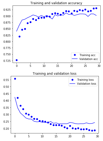
미세 조정
- 특성 추출에 사용했던 동결 모델의 상위 층 몇 개를 동결세어 해제하고 모델에 새로 추가한 층(여기선 완전 연결 분류기)과 함께 훈련하는 것
- 주어진 문제에 조금 더 밀접하게 재사용 모델의 표현을 일부 조정하기 때문에 미세 조정이라고 부른다.
네트워크 미세 조정하는 단계
- 사전에 훈련된 기반 네트워크 위에 새로운 네트워크를 추가한다.
- 기반 네트워크를 동결한다.
- 새로 추가한 네트워크를 훈련한다.
- 기반 네트워크에서 일부 층의 동결을 해제한다.
- 동결을 해제한 층과 새로 추가한 층을 함께 훈련한다.
# 특정 층까지 모든 층 동결하기
conv_base.trainable = True
set_trainable = False
for layer in conv_base.layers:
if layer.name == 'block5_conv1':
set_trainable = True
if set_trainable:
layer.trainable = True
else:
layer.trainable = False
모델 미세 조정
# 모델 미세 조정하기
model.compile(loss='binary_crossentropy',
optimizer = optimizers.RMSprop(lr=1e-5),
metrics=['acc'])
log = model.fit_generator(
train_generator,
steps_per_epoch=100,
epochs=100,
validation_data = validation_generator,
validation_steps=50
)
model.save('cats_and_dogs_small_4.h5')결과 그래프
# 결과 그래프 그리기

import matplotlib.pyplot as plt

acc = log.history['acc']
val_acc = log.history['val_acc']
loss = log.history['loss']
val_loss = log.history['val_loss']

epochs = range(1, len(acc) + 1)

plt.plot(epochs, acc, 'bo', label='Training acc')
plt.plot(epochs, val_acc, 'b', label='Validation acc')
plt.title('Training and Validation accuracy')
plt.legend()

plt.figure()

plt.plot(epochs, loss, 'bo', label = 'Training loss')
plt.plot(epochs, val_loss, 'b', label = 'Validation loss')
plt.title('Training loss and Validation loss')
plt.legend()

plt.show()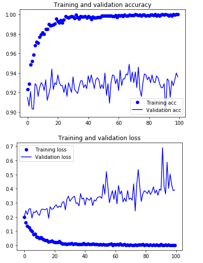
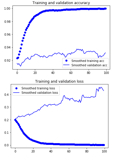
부드러운 그래프 그리기
#  부드러운 그래프 그리기

def smooth_curve(points, factor=0.8):
    smoothed_points = []
    for point in points:
        if smoothed_points:
            previous = smoothed_points[-1]
            smoothed_points.append(previous * factor + point * (1-factor))
        else:
            smoothed_points.append(point)
    return smoothed_points

plt.plot(epochs, smooth_curve(acc), 'bo', label = 'Smoothed training acc')
plt.plot(epochs, smooth_curve(val_acc), 'b', label = 'Smoothed validation acc')
plt.title('Trining and validation accuracy')
plt.legend()

plt.figure()

plt.plot(epochs, smooth_curve(loss), 'bo', label = 'Smoothed training loss')
plt.plot(epochs, smooth_curve(val_loss), 'b', label = 'Smoothed validation loss')
plt.title('Trining and validation loss')
plt.legend()

plt.show()
- 지수 이동 평균(exponential moving averages)으로 정확도와 손실 값을 부드럽게 표현할 수 있다.
모델 평가
# 모델 평가

test_generator = test_datagen.flow_from_directory(
    test_dir,
    target_size=(150,150),
    batch_size = 20,
    class_mode = 'binary'
)

test_loss, test_acc = model.evaluate_generator(test_generator, steps=50)
print('test acc : ', test_acc)
728x90
반응형


최근댓글